Optimization of Statistical Modeling Parameters for Geophysical Fields in Permafrost Conditions

Kambalin Igor' Olegovich Postgraduate student; Faculty of Geography; Lomonosov Moscow State University 119991, Russia, Moscow, Leninskie Gory str., 1 igorkambalin@gmail.com Other publications by this author     Koshurnikov Andrey Viktorovich ORCID: 0000-0001-6160-7795 Doctor of Geology and Mineralogy Lecturer; Department of Glaciology and Cryolithology; Moscow State University 119192, Russia, Moscow, Stoletova str., 9, sq. 12 koshurnikov@msu-geophysics.ru Other publications by this author

Balihin Ermolai Igorevich Postgraduate student; Faculty of Geology; Lomonosov Moscow State University 119234, Russia, Moscow, Leninskie gory str., 1 ermikus2@mail.ru Other publications by this author

Introduction

Methods of studying permafrost rocks remain an urgent problem in modern geophysics and geocryology. The reason for this, in many ways, is the limited number of techniques related to the choice of parameters for statistical modeling of geophysical data in the cryolithozone. In most cases, such parameters are chosen based on empirical assumptions, which makes it more difficult to obtain reasonable and reproducible results. This creates difficulties for researchers trying to adapt existing methods or develop new approaches for analyzing and predicting soil properties.

Parameterization of the environment in the cryolithozone requires an understanding of the directions and nature of the variability of the physical properties of rocks. Re-vein ices create a sharp contrast of properties laterally, while stratified ices cause vertical changes. Transitions between different types of soils, for example, from clay to rocks, also introduce vertical contrasts. Properties such as humidity, salinity, and waterlogging have a significant impact on the physical characteristics of the medium ^[1]. However, the lack of unified approaches to parameterization of physical properties for probabilistic modeling and interpolation leads to the fact that researchers often rely on limited or empirical data ^[2-4]. This reduces the accuracy of the models and makes it difficult to extrapolate the results obtained.

In such conditions, it becomes necessary to create complex methods combining data from geophysical research and advanced statistical models ^[5-7]. Modern technologies, including methods of three-dimensional statistical modeling ^[8], make it possible to more accurately account for the spatial variability of data. However, the success of their application depends on the correct selection of parameters, which often requires additional research and testing under specific geological conditions ^[9].

The research is aimed at finding optimal statistical modeling parameters that make it possible to create accurate spatial models of the distribution of the physical properties of permafrost rocks based on the integration of geophysics data. The following tasks are formulated for this purpose:

1. To provide an overview of statistical modeling methods, highlighting the most universal approaches, and briefly describe their advantages and limitations.

2. To analyze the effect of interpolation parameters (search radius, number of neighbors, type of covariance function) on the quality of three-dimensional models in difficult geological conditions.

3. To study Bayesian kriging methods and adapt them to the specifics of the cryolithozone with the formation of recommendations for their use.

4. To analyze the variability of the physical properties of soils, revealing the relationship with geomorphological and lithological features.

5. To validate the created models using data from drilling operations and field observations ^[10].

6. To develop algorithms for the integration of geophysical and drilling data, taking into account the specific features of the cryolithozone.

In the course of the work, the three-dimensional Bayesian kriging method used for interpolation of geophysical data was tested. The research was carried out on the territory of the slag heaps of the nickel plant in Norilsk, where a similar method had not been used before. The use of the three-dimensional Bayesian kriging method made it possible to identify patterns in the spatial distribution of the physical properties of permafrost rocks, as well as to study their variability.

5 spatial voxel models of the electrical resistivity field distribution with different approximation parameters are constructed. Based on these models, a set of 5 spatial maps and corresponding sections has been compiled, within the framework of which frozen strata have been interpreted and contoured, as well as an analysis of the correspondence of the selected strata to the actual core material of the wells.

Overview of statistical modeling methods

Statistical modeling is used to analyze large amounts of data, identify patterns, and predict geophysical fields. Modern mathematical methods and computational technologies make it possible to efficiently process multidimensional data and interpolate it in complex geological environments.

Statistical modeling methods can be subdivided according to their characteristic features ^{[11, 12]}:

By type of input data:

- spatial: kriging, spatial interpolation methods (IDW - Inverse Distance Weighing, spline functions);

- time series: time series analysis;

- multidimensional: cluster analysis, regression methods.

For the purposes of the analysis:

- interpolation: kriging, IDW, splines;

- classification: Random Forest, cluster analysis;

- regression: correlation and regression analysis;

- uncertainty assessment: Bayesian Methods, Bayesian kriging.

In terms of algorithmic complexity and requirements for the amount of data for calculations:

- the simplest: IDW, linear regression;

- complex: Gradient Boosting, Deep Learning, Bayesian Kriging.

Geophysical studies in the cryolithozone, complicated by the heterogeneity of the environment (variability of soil structure, variations in thermal conductivity, complex processes of freezing and thawing, high electrical conductivity of taliks along with increased electrical resistance of icy rocks, etc.), are most interesting for statistical modeling [Douglas, Zheng, Gruber, Jørgensen]. This is primarily due to the large amount of data obtained (unlike drilling data), as well as their ambiguity. That is, the data obtained by themselves can describe several geocryological situations at once, and additional studies are necessary for an unambiguous interpretation.

The following features and requirements for statistical models should be highlighted for geophysical research:

- geostatistical approaches should take into account the anisotropy of the physico-mechanical properties of frozen soils ^{[3, 13]};

- forecasting methods should be adapted to process data with gaps and high degree of noise;

Spatial interpolation requires taking into account local changes in the thermal field and other parameters, without separating them into a group of noises.

Bayesian 3D kriging, supplied in the ArcGIS Pro software package, is the most suitable method for working with geophysical data in the cryolithozone, as it meets the above requirements.

In comparison with other geostatistical methods such as IDW, splines, or classical kriging, Bayesian 3D kriging provides more accurate modeling of complex geophysical processes by accounting for uncertainty ^[14].

At the same time, Bayesian kriging differs from complex machine learning methods such as Random Forest or Gradient Boosting by having built-in mechanisms for accounting for spatial correlation and data anisotropy. Machine learning methods can also take into account the spatial relationships of the input data, especially Deep Learning algorithms, but this requires a large amount of training data and the embedding of energy-intensive modules, which take longer to calculate.

Determination of model construction parameters by Bayesian kriging method 3 D

In ArcGIS Pro, Bayesian 3D kriging provides the user with a set of parameters that can be configured to optimize the final model. The main settings include:

1. Selecting a field to account for measurement errors – when measuring the same parameter with different equipment for which measurement errors are known.;

2. A model of a semivariogram defining the form of spatial correlation of the initial data:

- power – This model describes a correlation that increases with distance but does not reach a threshold. It is useful for data with long correlation and gradual changes.;

- linear – the linear model assumes a proportional increase in variance with distance. It is used for data with linear correlation;

- thin Plate Spline – This model is suitable for data with high smoothness. It is often used for interpolation of complex surfaces.;

exponential – the exponential model works well with data where the correlation decreases rapidly with increasing distance;

- whittle is a model that is used for data with a more complex spatial structure, including anisotropy;

- K-Bessel is a model used to describe complex correlation structures that involve cyclical or repetitive processes.

3. Type of transformation – allows you to take into account the presence of outliers (values that differ sharply from the main data set) in the source data:

- none – used if the source data has no outliers or has been preprocessed.;

- empirical – smooths the data array if it contains outliers;

- log empirical – logarithmic empirical transformation is suitable for data with a wide range of values, avoiding unnecessary smoothing;

- subset size – sets the size of the subsample (local model) of data used to calculate local interpolation parameters. Increasing the size of the subsample reduces the number of subsamples, which can increase the stability of the model, as more points reduce the impact of outliers and noise. However, this can smooth out local variations. Reducing the Subset Size makes the model more adaptive to local features, but increases its sensitivity to noise and instability. However, reducing the size of the subsample leads to an increase in the number of such subsamples, which can increase the calculation time.

4. Local model area overlap factor – determines the degree of overlap between subsamples. Each data point can fall into several subsamples. Higher overlap factor values create a smoother output surface, as each point is processed several times. However, an increase in the overlap factor leads to an increase in calculation time. The parameter values should be between 1 and 5. The actual overlap is usually greater than the specified value to ensure the same number of points for each local model.

5. Number of simulated semivariograms – the number of semivariograms being constructed for each local model. The higher this number, the more stable the model will be, but this significantly increases the calculation time. The selection of this parameter primarily depends on the noise level of the data and usually lasts from 100 to 500 simulations. In order to check whether the selected quantity is sufficient, it is possible to estimate the prediction error in the constructed model. So, if the variance of the initial data is an order of magnitude greater than the standard error of the model, then the model can often be considered correct.

6. Order of trend removal – allows you to remove the trend of changing values vertically. This operation is often required if vertical measurements are performed much more frequently than horizontal measurements, which means that trends have a greater impact on the overall vertical smoothing of the model. To analyze local changes, such trends can be deleted, which will allow for greater variability of values vertically.:

- none – the trend is not deleted, this parameter is used by default.;

- first order – removes the first-order linear trend in the vertical direction, which helps to stabilize calculations and reduce the impact of strong vertical changes in values. This approach is useful for data that changes vertically faster than horizontally.

7. Elevation inflation factor – determines the scaling of values in the vertical direction before calculating the model and interpolating. This parameter corrects the difference in the variability of values vertically and horizontally, making one single step in height equivalent to one step horizontally. Higher parameter values enhance the influence of the vertical data structure, which stabilizes calculations and improves interpolation accuracy. The default value is calculated automatically using the maximum likelihood method and is usually in the range from 1 to 1000. The user can set their own value to refine the model based on cross-validation.

8. Search neighborhood – defines the neighbor search parameters for interpolation. This parameter has a number of settings that should also be considered.:

- max neighbors – the maximum number of neighboring points used to calculate the values. Increasing this parameter increases stability, but it can smooth out local details.;

- min neighbors – the minimum number of neighbors required to perform the calculation. Low values increase the flexibility of the model, but may impair stability in sparse data.

Sector type: Divides the space around a point into sectors (Platonic solids):

1) 1 Sector (Sphere): All nearest neighbors from any direction. A simple solution for uniform data.

2) 4 Sectors (Tetrahedron): Division into four sectors.

3) 6 Sectors (Cube): Division into six regions.

4) 8 Sectors (Octahedron): Dividing the space into eight sectors.

5) 12 Sectors (Dodecahedron): Dividing into 12 sectors for uniform space coverage.

6) 20 Sectors (Icosahedron): Division into 20 sectors for a more detailed neighbor search.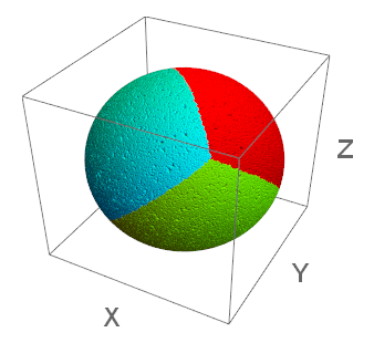

Fig. 1. An example of dividing the search area into 4 sectors [Esri. 3D Search Neighborhoods. URL: https://pro.arcgis.com/ru/pro-app/latest/help/analysis/geostatistical-analyst/3d-search-neighborhoods.htm (date of request: 10.12.2024)]

During the configuration of the model itself, you can choose how points with matching coordinates will be processed, which can be useful if you perform a double measurement to verify the data you receive. In the Coincident Points environment setting, you can set the following parameters:

- mean of values at coincident locations (default) – for all matching points at the same location, the average value is calculated;

- exclude all coincidental data – completely excludes all coincidental points from the analysis;

- minimum value at coincident locations – uses the minimum value of all matching points at a given location;

- include all coincidental data – all data on coincidental points is included in the analysis without averaging or exclusion.

Selection of parameters for Bayesian 3-D kriging using the example of frequency sensing data

To refine the data selection method, data on electrical resistivity obtained by frequency sensing at a landfill near the slag heap of the city of Norilsk is used (Fig. 2). The data includes 11 profiles, the distance between which is 100 meters, and the frequency of profile survey is every 2 meters. The total number of points is 69,076. During data processing, each point was assigned XY coordinates based on the GPS tracker built into the equipment, and the Z coordinate was assigned as the difference between the integral depth of measurement and the height of the point on the digital terrain model. The digital model was based on pre-classified points, excluding points of high and low vegetation, as well as reservoirs.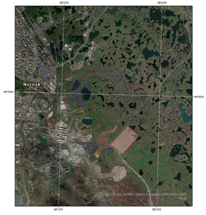

Fig. 2. Contour of the survey site

Within the studied territory, re-vein ice is widespread, the predominant composition of sediments is represented by tundra gley-peat and peat (peat and peat tundra gley soils) soils lying on clay and heavy loamy gravelly rocks ^{[15, 16]}.

Studies have been conducted at the landfill aimed at mapping anthropogenic pollution by metal particles blown off the landfill and decomposing at the site ^[9].

In order to build a spatial model of the distribution of electrical resistivity, we will form the requirements for the desired model, taking into account the available data on the environment.:

1. The measured data, based on the knowledge of the environment and the preliminary analysis of points at the stage of in-house processing, are subject to significant anisotropy of properties. This is primarily due to the fact that the electrical resistance depends on both the lithological composition (and the presence of metallic contamination) and the phase state of the water in the soil. If the former has the greatest lateral variability, then the latter has the greatest variability with depth. It is necessary to select a type of variograms for modeling that is suitable for data with pronounced anisotropy, namely, Whittle.

2. There is a fairly large number of values significantly exceeding the modulo weighted average value, which indicates the need to choose the type of transformation not None.

3. The data is located close enough to each other within the profile, but not between profiles, and the network is not uniform. Let's take the Elevation Inflation Factor to be 10, which reflects the ratio of the distance between the profiles to the depth of the method. At the same time, the radius of the neighbor search must be greater than the distance between the profiles by a factor of 1-1.5.

4. The data is not uniform in all directions due to the non-isometric network. To account for this fact, you should take a Sector type no smaller than a Cube (more than 4 sectors).

We will select the number of minimum and maximum neighbors, as well as the number of simulations, based on empirical considerations, as well as the power of the available computing equipment.

Thus, 5 models were created that make it possible to visually assess the difference in the application of various parameters (Tables 1, 2).

Table 1

Table 2

Based on the obtained 3D voxel models of the distribution of electrical resistivity fields, a set of maps and sections has been created (Fig. 3-7), on which the obtained fields are interpreted and tested using test drilling operations. The images below show the results of three-dimensional statistical modeling of the distribution of the geoelectric properties of permafrost rocks using various Bayesian kriging parameters.

Figure 3. Model (No. 1) of the distribution of the geoelectric properties of permafrost rocks. Map and section

Figure 4. Model (No. 2) of the distribution of the geoelectric properties of permafrost rocks. Map and section

Figure 5. Model (No. 3) of the distribution of the geoelectric properties of permafrost rocks. Map and section

Figure 6. Model (No. 4) of the distribution of the geoelectric properties of permafrost rocks. Map and section

Figure 7. Model (No. 5) of the distribution of the geoelectric properties of permafrost rocks. Map and section

Let's look at the results obtained in more detail, comparing the various model options and their correspondence to the actual drilling data for wells No. 5, 6 and 8.

Well No. 5 is located on the northern slope of a natural elevation, which ensures stable rock freezing. The core contains light loams and heavy sandy loam with a massive cryostructure, which cause high electrical resistance.

Models No. 4 and No. 1 do not detect thawed rocks to depths of 20 meters, although they allow us to judge a slight decrease in resistance in the vicinity.

Models No. 5 and No. 2, although they reflect the position of the meltwater quite close to reality, are not reliable enough. In model No. 2, the values for the thickness of the thawed layer turned out to be overestimated, and the roof of the thawed layer was found to be 0.4 m higher than in reality. And in model No. 5, the borders turned out to be smoothed out and no longer reflect the natural state of the environment, but the transitions between individual areas.

Model No. 3, in turn, most accurately corresponds to the actual core data, showing a thawed layer already at a depth of about 17.5 m, confirming the high accuracy of the exponential semivariogram and the adequacy of the neighbor search parameters (15 points, 6 sectors). Moreover, the nature of the field distribution in the vicinity of well No. 5 is more clearly displayed precisely within the framework of model No. 3, reflecting the structure consistent with the exposure conditions.

The environment within well No. 8 is also characterized by consistently high resistance at almost the entire depth due to the presence of frozen light loams and sandy loams. However, due to the lower ice content, the contrast of the medium near this well is lower than near well No. 5. None of the models can demonstrate absolute accuracy in the results obtained. However, it turned out to be the closest to reality to outline the boundary of the thawed layer within the framework of model No. 3 at a depth of 18.4 m, which only slightly does not correspond to the actual position of the boundary (18.7 m). The remaining models show either underestimated values (model No. 1) or overestimated values (models No. 4 and 2), reflecting the boundary at a depth of only 16.0–16.5 m. Model No. 5 hallucinated the appearance of a high–resistance layer under the frozen layer at depths of 18.0-20.0 m.

Well No. 6 shows the opposite picture, with a predominance of low-resistance rocks, which is not confirmed by drilling, which revealed light loams with an incomplete lattice cryostructure.

Upon further analysis, it was revealed that the brown color of the sediments and the abnormally low electrical resistivity indicate the burial of metal waste in this place. This feature is clearly recorded by all models, but model No. 3 again demonstrates the most detailed and structured display of the low-resistance layer, which is important for assessing the extent of pollution.

Advantages of using Model No. 3:

1. High accuracy of mapping the soles of frozen rocks and the presence of thawed layers, confirmed by core data.

2. Good compliance with the actual observations on the boundaries of zones of different ohms.

3. Resistance to noise and local anomalies.

Disadvantages of other models:

1. Model No. 1 shows a weak correspondence to the actual data in areas of sharp boundaries.

2. Models No. 2 and No. 4 are less detailed and often smooth out important details.

3. Model No. 5, despite its high level of detail, shows increased sensitivity to noise and instability in reflecting small-scale anomalies.

Thus, the optimal choice for statistical modeling in these conditions is model No. 3 with an exponential semivariogram, logarithmic empirical transformation and a moderate number of sectors. The results confirmed by core observations allow us to recommend this model for similar studies in the cryolithozone.

Moreover, the use of the method of selecting modeling parameters based on the features of the geocryological structure really allows you to achieve the most accurate results in modeling, and the wrong choice due to insufficient study of the environment leads to errors that can potentially adversely affect the course of engineering and geological work in the territory ^{[17, 18]}.

References

1. Akimov, A. T., Klishees, T. M., Melnikov, V. P., & Snegirev, A. M. (1988). Electromagnetic methods of permafrost research (V. D. Badalov, Ed.). Institute of Permafrost Studies.
2. Eltsov, I. N., Olenchenko, V. V., & Fage, A. N. (2017). Electrical tomography in the Russian Arctic based on field research data and three-dimensional numerical modeling. Neftegaz.RU, 2, 54-64.
3. Ershov, E. D. (2002). General geocryology. Moscow State University Press.
4. Sudakova, M. S., Brushkov, A. V., Velikin, S. A., Vladov, M. L., Zykov, Y. D., Neklyudov, V. V., Olenchenko, V. V., Pushkarev, P. Y., Sadurtdinov, M. R., Skvortsov, A. G., & Tsarev, A. M. (2022). Geophysical methods in geocryological monitoring. Moscow University Bulletin. Series 4. Geology, 6.
5. Shesternyov, D. M., & Omelyanenko, P. A. (2018). Increasing the efficiency of engineering and geophysical methods in studying permafrost soils. Bulletin of Transbaikal State University, 5, 1184-1196.
6. Kosticyn, V. I., & Khmelevskoy, V. K. (2018). Geophysics: textbook. Perm National Research University.
7. Herring, T., Lewkowicz, A. G., Hauck, C., et al. (2023). Best practices for using electrical resistivity tomography to investigate permafrost. Permafrost and Periglacial Processes, 34(4), 494-512.
8. Yaitsikaya, N. A., & Brigida, V. S. (2022). Geoinformation technologies in solving three-dimensional geoecological problems: spatial data interpolation. Geology and Geophysics of Southern Russia, 12(1), 162-173.
9. Kambalin, I.O., Koshurnikov, A.V., Balihin, E.I. (2024). The Role of Digital Elevation Models in Increasing the Accuracy of Geophysical Studies of Anthropogenic Metallic Pollution. Arctic and Antarctica, 4, 13-23. https://doi.org/10.7256/2453-8922.2024.4.71872
10. Douglas, T. A., Hiemstra, C. A., Anderson, J. E., et al. (2021). Recent degradation of interior Alaska permafrost mapped with ground surveys, geophysics, deep drilling, and repeat airborne lidar. The Cryosphere, 15(8), 3555-3571.
11. Dolgal, A. S., Muravina, O. M., Auzen, A. A., Ponomarenko, I. A., & Gruzdev, V. N. (2019). Areas of application of modern statistical methods for processing geophysical information. Bulletin of VSU. Series: Geology, 4, 79-84.
12. Osipov, V. V. (2011). Analysis of methods for creating digital surface models. GEO-Siberia-2011 (Vol. 1, Part 2, pp. 82-86). Proceedings of the VII International Scientific Congress "GEO-Siberia-2011," April 19-29, 2011, Novosibirsk. SGGA.
13. Vegter, S., Bonnaventure, P. P., Daly, S., & Kochtitzky, W. (2024). Modelling permafrost distribution using the temperature at the top of permafrost (TTOP) model in the boreal forest environment of Whatì. Arctic Science, 10(3), 455-475.
14. Treat, C. C., Virkkala, A.-M., Burke, E., Bruhwiler, L., Chatterjee, A., Hayes, D. J., et al. (2024). Permafrost carbon: progress on understanding stocks and fluxes across northern terrestrial ecosystems. Journal of Geophysical Research: Biogeosciences, 129(2).
15. Geological map of Quaternary deposits: R-45 (Norilsk). State geological map of the Russian Federation. Third generation. Norilsk series. Map of Quaternary formations, scale: 1:1,000,000 (V. A. Radyko, Ed.). FGUP "VSEGEI."
16. Paderin, P. G., Demenyuk, A. F., Nazarov, D. V., Chekanov, V. I., et al. (2016). State geological map of the Russian Federation. Scale 1:1,000,000 (third generation). Norilsk series. Sheet R-45-Norilsk. Explanatory note. Cartographic factory VSEGEI.
17. Jorgenson, M. T., & Grosse, G. (2022). Remote sensing of landscape change in permafrost regions: progress, challenges, and opportunities. Permafrost and Periglacial Processes, 33(4), 429-447.
18. Overduin, P. P., Wegner, C., Kassens, H., et al. (2021). Subsea permafrost dynamics and coastline retreat in the Arctic shelf: statistical modeling of observations. Geosciences, 11(12), 505.
Peer Review
Peer reviewers' evaluations remain confidential and are not disclosed to the public. Only external reviews, authorized for publication by the article's author(s), are made public. Typically, these final reviews are conducted after the manuscript's revision. Adhering to our double-blind review policy, the reviewer's identity is kept confidential.
The list of publisher reviewers can be found here.
The subject of the study is the optimization of the parameters of statistical modeling of geophysical fields in cryolithozone conditions. The relevance of the study is obvious, since the author correctly states that "methods for studying permafrost rocks remain an urgent problem in modern geophysics and geocryology. The reason for this, in many ways, is the limited number of techniques related to the choice of parameters for statistical modeling of geophysical data in the cryolithozone. In most cases, such parameters are chosen based on empirical assumptions, which makes it more difficult to obtain reasonable and reproducible results. This creates difficulties for researchers trying to adapt existing methods or develop new approaches for analyzing and predicting soil properties. In such conditions, it becomes necessary to create complex methods that combine data from geophysical research and advanced statistical models. Therefore, the author's research is aimed at finding optimal statistical modeling parameters that make it possible to create accurate spatial models of the distribution of the physical properties of permafrost rocks based on the integration of geophysics data. The research methodology is based on statistical modeling methods, Bayesian kriging methods and their adaptation to the specifics of the cryolithozone, spatial interpolation methods (IDW - Inverse Distance Weighing, spline functions), Random Forest, cluster analysis, correlation and regression analysis, algorithms for integrating geophysical and drilling data. The scientific novelty lies in the fact that the research was carried out on the territory of the slag heaps of the nickel plant in Norilsk, where a similar method had not been used before. As a result of the study, 5 spatial voxel models of the distribution of the resistivity field with various approximation parameters were constructed, a set of 5 spatial maps and corresponding sections was compiled, within which the frozen strata were interpreted and contoured. The style of the article is scientific. The article is very informative, provided with tabular and illustrative material, which gives it a significant advantage. However, the structure of the article does not fully meet the established requirements of the journal, so it is recommended to highlight the sections "Research results" and "Conclusions" in it. In terms of volume and bibliography, the article meets the requirements of the journal. There are technical typos in some sentences (for example, in the last paragraph before the section "Overview of statistical modeling methods", the words "appropriate" and "interpreted" should be written as "appropriate" and "interpreted". The bibliography of the article includes 18 literary sources, 6 of which are in a foreign language. The conclusions in the article are concise and convey the main idea of the author based on the research results. The author concludes that the optimal choice for statistical modeling in these conditions is model No. 3 with an exponential semivariogram, logarithmic empirical transformation and a moderate number of sectors. The results confirmed by core observations allow us to recommend this model for similar studies in the cryolithozone. The appeal to the opponents consists in references to the literary sources used and the expression of the author's opinion on the problem under study. The reviewed article will undoubtedly be interesting and useful to scientists and practitioners of soil and permafrost studies, since the use of the method of selecting modeling parameters based on the features of the geocryological structure really allows you to achieve the most accurate results in modeling, and the wrong choice due to insufficient study of the environment leads to errors that can potentially adversely affect the course of engineering and geological work on territories. This article is recommended for publication in the journal "Arctic and Antarctic" after minor revision.